
This is a guest post by Yonatan Hadar. He is a data scientist with a machine and deep learning experience in Natural language processing, Time series analysis, Recommendation engines, and more domains. He is currently working as a data scientist at BigPanda and studying for a master’s degree at TAU big data lab.
Last month I started my new data science job at BigPanda and after a few days of installations, lectures and meeting new people I finally got access to the data. As an educated data scientist that always works according to CRISP-DM, I wanted to start my project with an exploratory data analysis (EDA). I usually do EDA on tabular data by using histograms, bar plots, a correlation matrix, scatter plots and other tools but none of these tools were suitable for textual data — which is the main data type at BigPanda.
In this blog post, I’m going to review several methods I used to get to know the textual data in the data exploration phase with code examples.
I will use a dataset of Donald Trump tweets from Kaggle for demonstration.
First of all, see some examples!
The first thing I do in every new data exploration is looking at the data. I want to feel out some basic questions about the text: Do I need a special pre-processing method? Are there any special characteristics? If there are labels, can I understand the label from the text or do I need more knowledge on the domain? Can I already spot special patterns in the data? Is there a connection to other variables in the data?
In the Trump dataset, we can see some Twitter specifics (ie: hashtags and usernames) and many URLs that we probably want to remove.
The Analysis
Now, on to the good stuff!
We’ll start the analysis with very simple text data statistics like text length and word frequencies. After that, we’ll investigate more sophisticated text characteristics using unknown words and feature engineering. Finally, we’ll use a machine learning-based topic modeling method to create semantic features from the text and assess the text in the context of time series analysis.
Basic statistics on the text
Text length
The length of the samples in the dataset is very important, as it can affect how you represent your text as features for the ML models. For example, TF-IDF is usually too sparse for short texts and average Word2Vec is usually too noisy for long texts.
The length can also affect the algorithm you use. For example, LSTM networks are much better than vanilla RNN networks on long texts.
We calculate the number of words in each tweet and look at the length distribution.
lens = data.Tweet_Text.str.split().apply(lambda x: len(x))
print(lens.describe())
lens.hist()
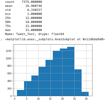
Results of this calculation establish that text length is short (average length of 17 words) but not very short (less than 10% has less than 5 words).
Term frequencies
In this step, I find the most frequent words in the data, extracting information about its content and topics.
When doing your analysis, remember to add domain-specific stop words, not just the known English stop words. I remove stop words from this particular analysis because they appear often but are not very informative.
from sklearn.feature_extraction.text import CountVectorizer
from nltk.corpus import stopwords

stops =  set(stopwords.words('english')+['com'])
co = CountVectorizer(stop_words=stops)
counts = co.fit_transform(data.Tweet_Text)

pd.DataFrame(counts.sum(axis=0),columns=co.get_feature_names()).T.sort_values(0,ascending=False).head(50)
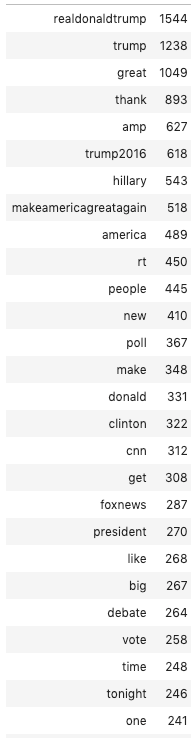
The top words are mostly campaign-related words, ie: Trump, Hillary, America, vote, poll, etc.
Now we can check for frequent bi-grams:
co = CountVectorizer(ngram_range=(2,2),stop_words=stops)
counts = co.fit_transform(data.Tweet_Text)
pd.DataFrame(counts.sum(axis=0),columns=co.get_feature_names()).T.sort_values(0,ascending=False).head(50)
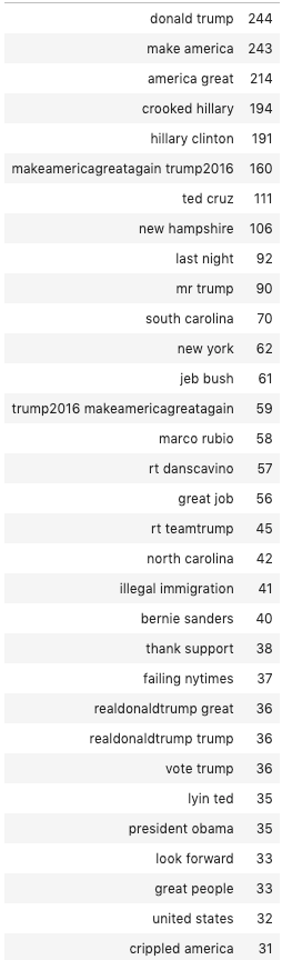
The most popular bi-grams are Trump’s special phrases, like “crooked Hillary” and “failing NYTimes”. There are also many mentions of competitors in the bi-grams (Hillary Clinton, Ted Cruz, Marco Rubio). This already gives us information about the differences in sentiment towards specific entities in the text.
More Sophisticated Text Characteristics
Unknown words
In this step, I search the text for elements like:
- Unknown words or words that don’t match known word lists.
- Words that appear especially often.
- How much of the text is slang?
- Which words are Domain-specific
- How many spelling mistakes appear in the text.
We can also find more steps to our preprocessing that will yield a better percentage of known words. This step is critical if you want to use pre-trained embeddings or pre-trained networks. In these cases, we need to compare the text data to the dictionary of the pre-trained resource.
In this analysis, I will use an English word list from https://github.com/dwyl/english-words and pre-process the text by removing hashtags, usernames and non-alphanumeric symbols.
words = pd.read_table('https://raw.githubusercontent.com/dwyl/english-words/master/words.txt')
words.columns=['word']
words = words['word'].str.lower().values.tolist()

data['clean_text'] = data.Tweet_Text.apply(lambda x: ' '.join([i for i in x.split(' ') if not (i.startswith('@') or i.startswith('#'))]))
data['clean_text'] = data.clean_text.str.lower().str.replace('[^a-zA]', ' ')
non_list = {}

for sent in tqdm(data.clean_text.str.split().values):
  for token in sent:
    if token not in words:
      non_list[token] = 1 if token not in non_list else non_list[token]+1

pd.Series(non_list).sort_values(ascending=False).head(30)
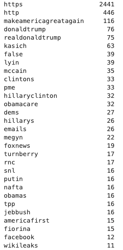
We probably need to add ״http” and ״https״ to the stop words (domain-specific stop words) list because they are frequent but not significant. Moreover, mostly names and bigrams were united (maybe we need a smarter tokenizer). Stemming or lemmatization can also help with removing more unknown words.
Feature engineering
It is possible to build some structure from the text by extracting features and then using the tools for structured data (histograms, bars, etc) on the features. Even though these features are very domain-specific, we can extract different types of entities or the sentiment of a sentence as features for almost every text dataset.
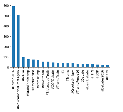
Here is a bar graph using hashtag frequency as features.
data.Tweet_Text.str.extractall(r'(\#\w+)')[0].value_counts().head(20).plot.bar()
Using machine learning models
Topic modeling
Topic modeling is a group of unsupervised machine learning methods aimed to extract meaningful topics from a text corpus. Topic modeling is helpful in exploring a new text dataset and understanding the different types of text samples. We can also use regular clustering but topic modeling is more interpretable and thus better for exploration.
I use the Latent Dirichlet Allocation algorithm with 10 topics and print the most important words in every topic.
from sklearn.decomposition import LatentDirichletAllocation, NMF

vectorizer = CountVectorizer(stop_words=stops)
model = vectorizer.fit(data.clean_text)
docs = vectorizer.transform(data.clean_text)

lda = LatentDirichletAllocation(20)
lda.fit(docs)

def print_top_words(model, feature_names, n_top_words):
  for topic_idx, topic in enumerate(model.components_):
    message = "Topic #%d: " % topic_idx
    message += " ".join([(feature_names[i])
    for i in topic.argsort()[:-n_top_words - 1:-1]])
      print(message)
  print()

print_top_words(lda,vectorizer.get_feature_names(),10)
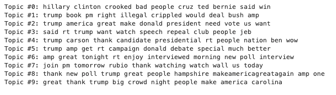
Here we see some clear topics. For example, Topic #0 about competitors, Topic #9 about rallies and Topic #2 about the campaign phrases:
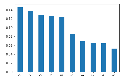
Now we assess how often Trump tweets about each topic:
data['topic']=lda.transform(docs).argmax(axis=1)
data.topic.value_counts(normalize=True).plot.bar()
And we can look at examples of specific topics:
data[data.topic==0].Tweet_Text.sample(5).values

Time series analysis
In many applications, our text corpus is associated with a time series (ie: news, tweets, reviews, etc.). Here we investigate the connection of the text to the time series. Now that we’ve built a text structure using the topic modeling, we can look at the topic distribution on the time series. We can also use time series anomaly detection and time series clustering methods to gain more insights on the topics.
data['Date']=pd.to_datetime(data.Date,yearfirst=True)
data.index = data.Date

for i in range(10):
  temp = data[data.topic==i]
  temp.resample('7D').size().plot()
  plt.title('topic %s' %i)
  plt.show()
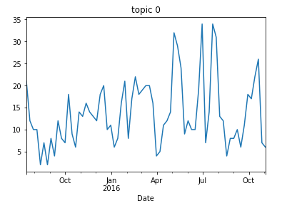
Topic #0 (competition) has 3 significant anomalies in May-August, there are suddenly over 30 tweets a week on the same topic.
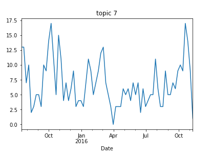
Topic #7 (radio and TV) has an interesting structure — in April it decreases drastically, gradually increasing until November. This makes sense because it represents two election periods, the republican primaries election and the US presidential election.
Conclusions
These methods really helped me get to know my text data, find the issues that needed attention and gain insight on how to appropriately use machine learning models on data. I hope it helps you, too!
Original. Reposted with permission.